We write a lot about why dashboards need honest pipelines underneath them. This post shows what that actually looks like, end to end, with screenshots of every layer — no whiteboard architecture, the real running system.
The subject is Global Bites, a five-store restaurant chain operating across four time zones: Mumbai, Bangalore, New York, Perth, and London. Eighteen months of operations — roughly 1.5 million rows covering the full supply chain, from ingredient sourcing and inventory through recipes, wastage, and per-counter sales — land in one MyRocks database per store (MySQL running the RocksDB storage engine; more on that choice below). The data is deliberately imperfect: duplicate sales, late-arriving dimensions, naive timestamps, schema drift, and unit mix-ups are seeded throughout, with a ground-truth manifest recording exactly what was injected, so the pipeline's cleaning can be scored rather than assumed.
One constraint made the exercise sharper: every tool is free and open-source. Apache Airflow for orchestration, Python for extraction, Parquet for the bronze layer, dbt Core on DuckDB for the warehouse, and Apache Superset for BI. No managed services, no per-seat licences — the whole platform runs on a laptop or a modest VM.
The source layer: MyRocks, built for the hyperscale write path
The operational store is deliberately not vanilla MySQL. Each store's database runs on MyRocks — MySQL on the RocksDB storage engine, served by Percona Server 8.0 in a Linux container — with every table declared ENGINE=ROCKSDB. Five shard-like databases, gb_mum through gb_lon, one per restaurant.
In one line: RocksDB — a fork of Google's LevelDB, maintained by Meta — delivers exceptionally fast write and read operations, especially on NVMe and SSD drives, and MyRocks is simply MySQL running on that RocksDB engine. The same engine shows up wherever scale is serious: it underpins storage at Meta and drives the state stores inside Kafka Streams, Apache Flink, and distributed databases like TiKV and YugabyteDB.
MyRocks exists because of a hyperscaling problem: it was built at Facebook to run MySQL's workload on a log-structured merge-tree engine instead of InnoDB's B-trees. An LSM engine absorbs writes into in-memory memtables and flushes them to disk as sorted, sequential files, rather than updating index pages in place — so write amplification drops sharply and sustained ingest stays fast as volume grows. The on-disk format also compresses far better than B-tree pages, which is exactly the trade a write-heavy, append-mostly workload like a POS feed wants: our 1,482,741 generated rows occupy roughly 251 MiB on disk, compressed by RocksDB, with per-schema sizes reported straight from the engine's information_schema tables.
Crucially, MyRocks keeps the MySQL surface: the extractor needs no special driver or change-data-capture magic, just an incremental SELECT keyed on the ingestion watermark. Hyperscale storage underneath, boring SQL on top.
The choice also comes with honest trade-offs, and they shaped the pipeline. MyRocks does not enforce foreign keys — relationships are logical only — and it runs READ COMMITTED rather than gap-locked repeatable reads. That is not a defect to paper over; it is how hyperscale operational stores actually behave: referential integrity moves out of the storage engine and into the pipeline, where dbt relationship tests own it. The injected referential breaks in the dataset land exactly on that seam, and the staging layer catches them.
Five restaurants is small, but the shape is what matters: a shard-per-store layout is how this scales to five thousand stores without redesign. The extract stage already fans out one task per database — more stores means more parallel extracts feeding the same bronze layer, and nothing downstream has to care how many shards exist.
The architecture in one paragraph
The design is a classic medallion flow. A Python extractor pulls each store's MyRocks database incrementally into bronze Parquet files, using an ingestion watermark so a rerun with no new data extracts nothing. dbt Core then builds the warehouse on DuckDB: staging views that clean and deduplicate, dimensional marts that carry the P&L from store level up to a consolidated global view, and an ops layer that watches the pipeline itself. Airflow schedules the whole thing daily and treats dbt's tests as the quality gate. Superset reads the finished gold layer and serves seven dashboards.
Orchestration: one DAG, five stores in parallel
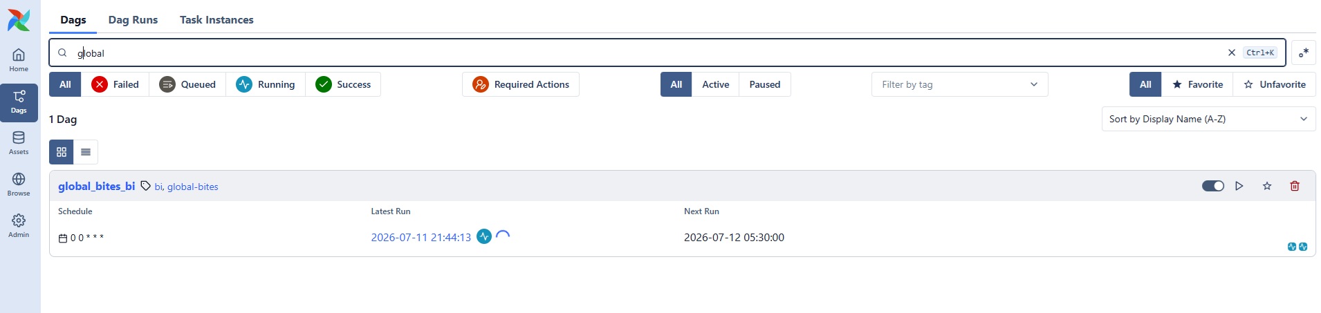
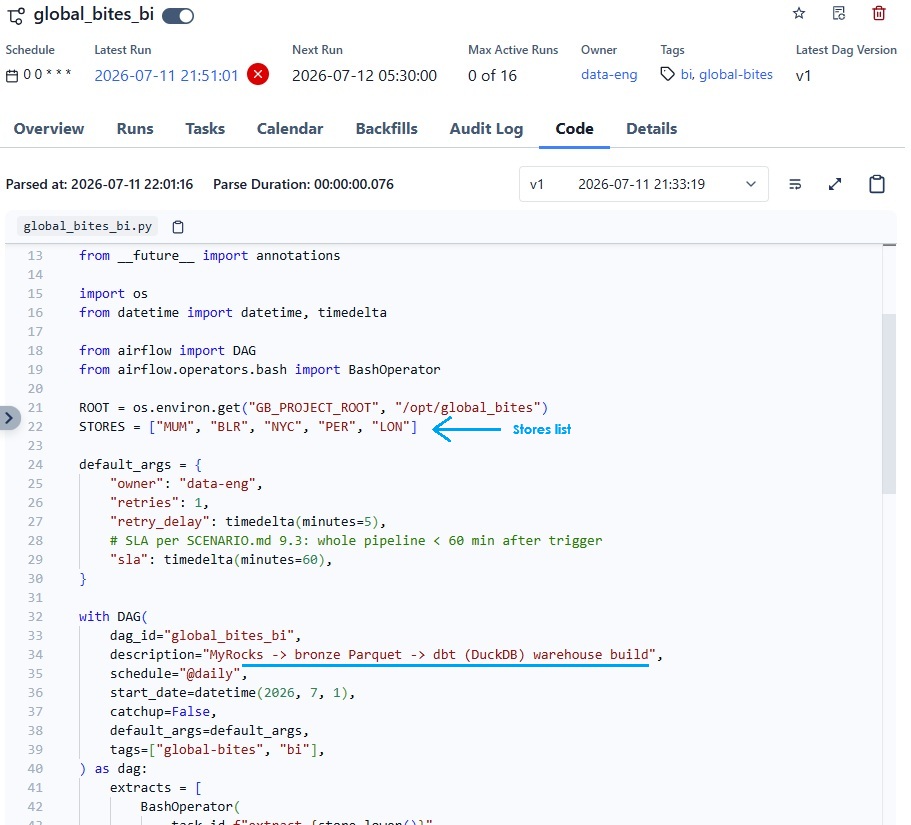
Everything hangs off a single Airflow DAG, global_bites_bi, scheduled daily with a 60-minute SLA. The Airflow home screen shows the operational contract at a glance: the schedule, the latest run, and the next one due.
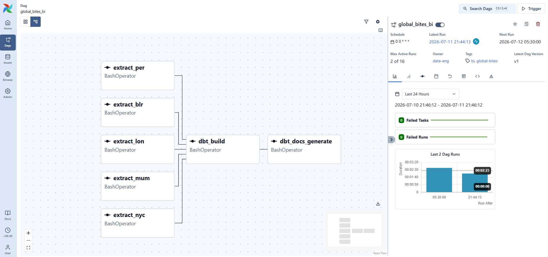
The graph view is where the shape of the pipeline becomes obvious. Five extract tasks — one per store — run in parallel, then fan in to a single dbt build, which is followed by documentation generation. Because the stores are independent, there is no reason for Perth to wait for Mumbai; parallel extraction keeps the wall-clock time close to the slowest single store rather than the sum of all five.
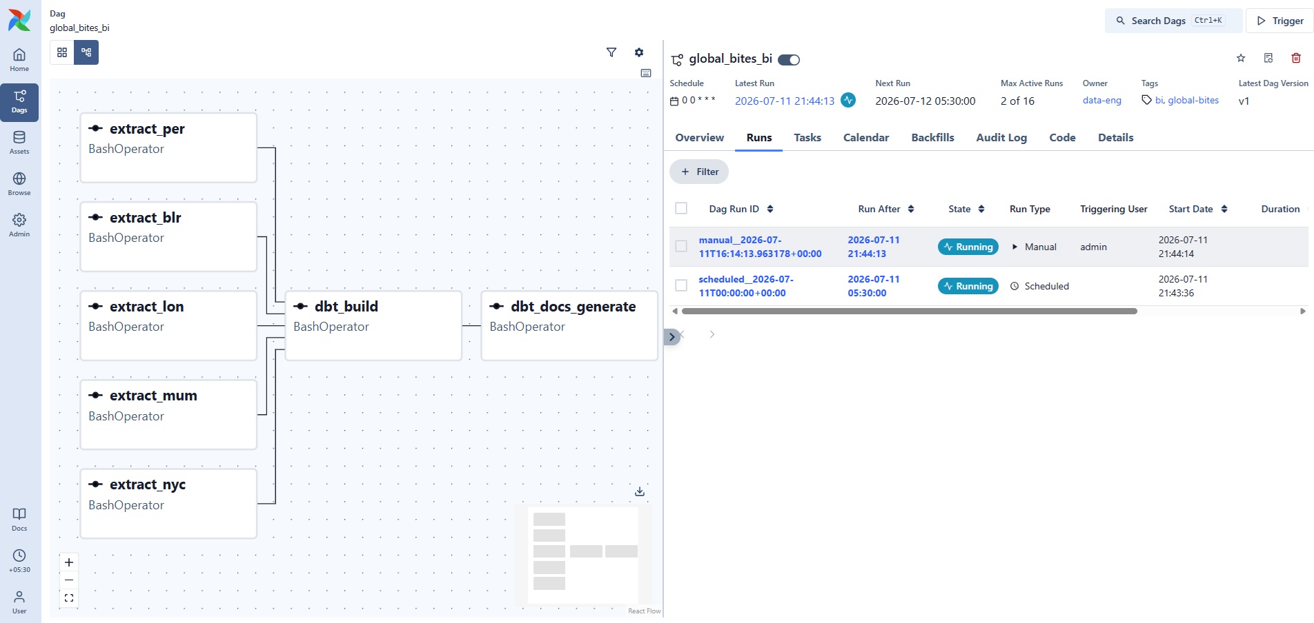
The Runs tab keeps the full history — scheduled runs beside manual ones, each with its trigger, state, and timing. This is the difference between "the pipeline ran" as a feeling and as a fact.
The whole DAG is about seventy lines of Python
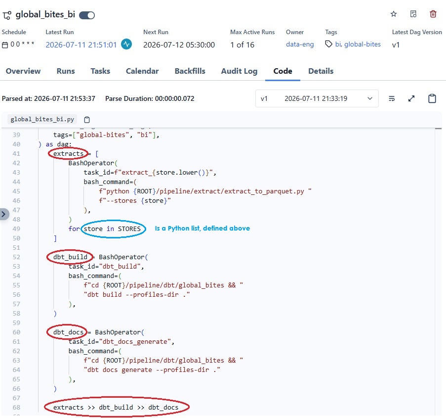
Orchestration code has a tendency to sprawl. This DAG stays small because it only orchestrates — every task is a thin BashOperator around a command you could run by hand, which means the pipeline can always be driven manually when you need to debug a single stage. The docstring states the contract up front: extract incrementally, build the warehouse, and let a failing dbt test fail the DAG.
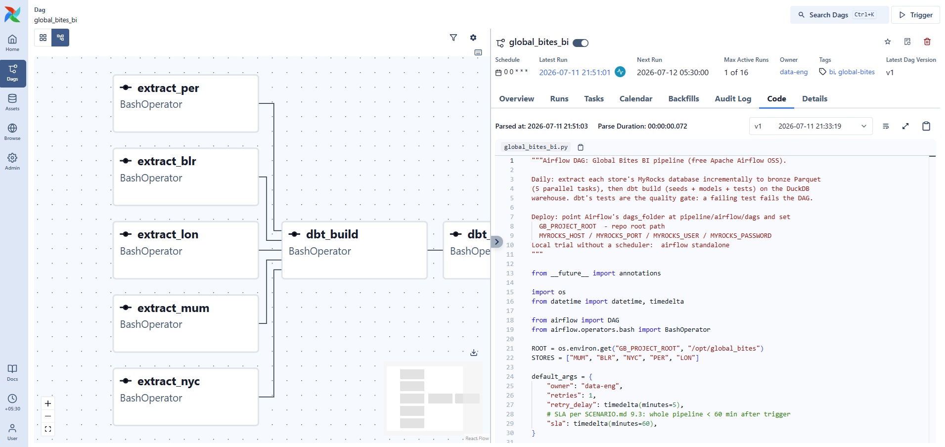
Configuration is explicit and boring, in the best way: the store list is a plain Python list, retries and the SLA live in default_args, and paths come from environment variables rather than hard-coded strings.
The tasks themselves are a list comprehension over the stores, and the dependency structure is a single line: extracts >> dbt_build >> dbt_docs. When the topology is this readable, code review of a pipeline change takes minutes.
Failure is expected — and handled
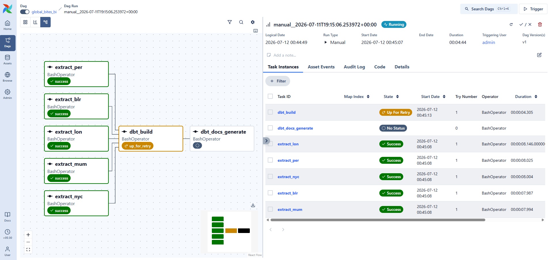
The most convincing screenshot in this whole post might be an amber one. During one run, dbt_build hit a transient failure; Airflow marked it up_for_retry and the downstream docs task simply waited. Nobody was paged, nothing was rerun by hand.
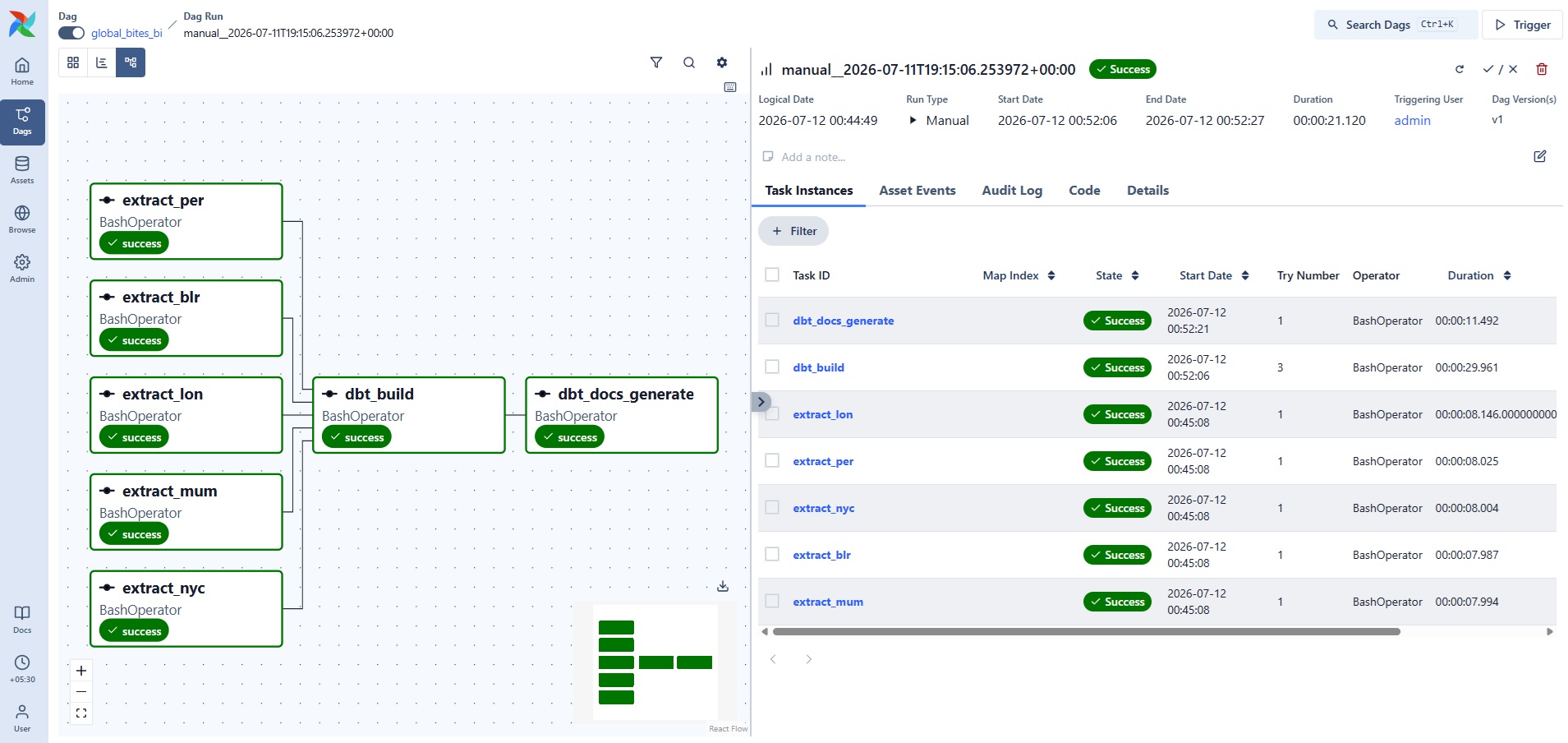
The retry succeeded — the same run finished green, with the task instance log showing it took three attempts. This is what "retries built into the schedule" means in practice: transient failures are absorbed by the platform instead of becoming somebody's morning.
The safety works in both directions. Retries absorb transient failures, but a genuine data problem must not be retried into production: dbt's tests run inside dbt_build, so bad data fails the DAG before anything downstream can consume it.
The warehouse is code: dbt on DuckDB
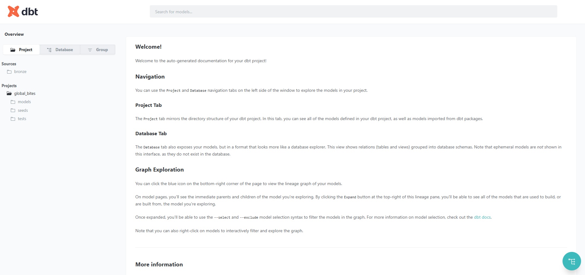
The warehouse itself is 33 dbt models and 35 tests, organised into staging, marts, and an ops layer, with two seeds for reference data. dbt generates a browsable documentation site from the project on every run — the same lineage and column documentation an analyst would otherwise have to reverse-engineer from SQL files.
Staging is where the injected mess gets cleaned: deduplication on natural keys, money-string and payment normalisation, timezone reconstruction for Perth's naive timestamps, SCD2 ranges for late-syncing dimensions, and kg-to-gram unit fixes. The marts above it carry the business logic — store and menu-item dimensions, sales facts, and a P&L that rolls up from store level through regional currency views to a consolidated global statement in USD, using an fx_rates seed.
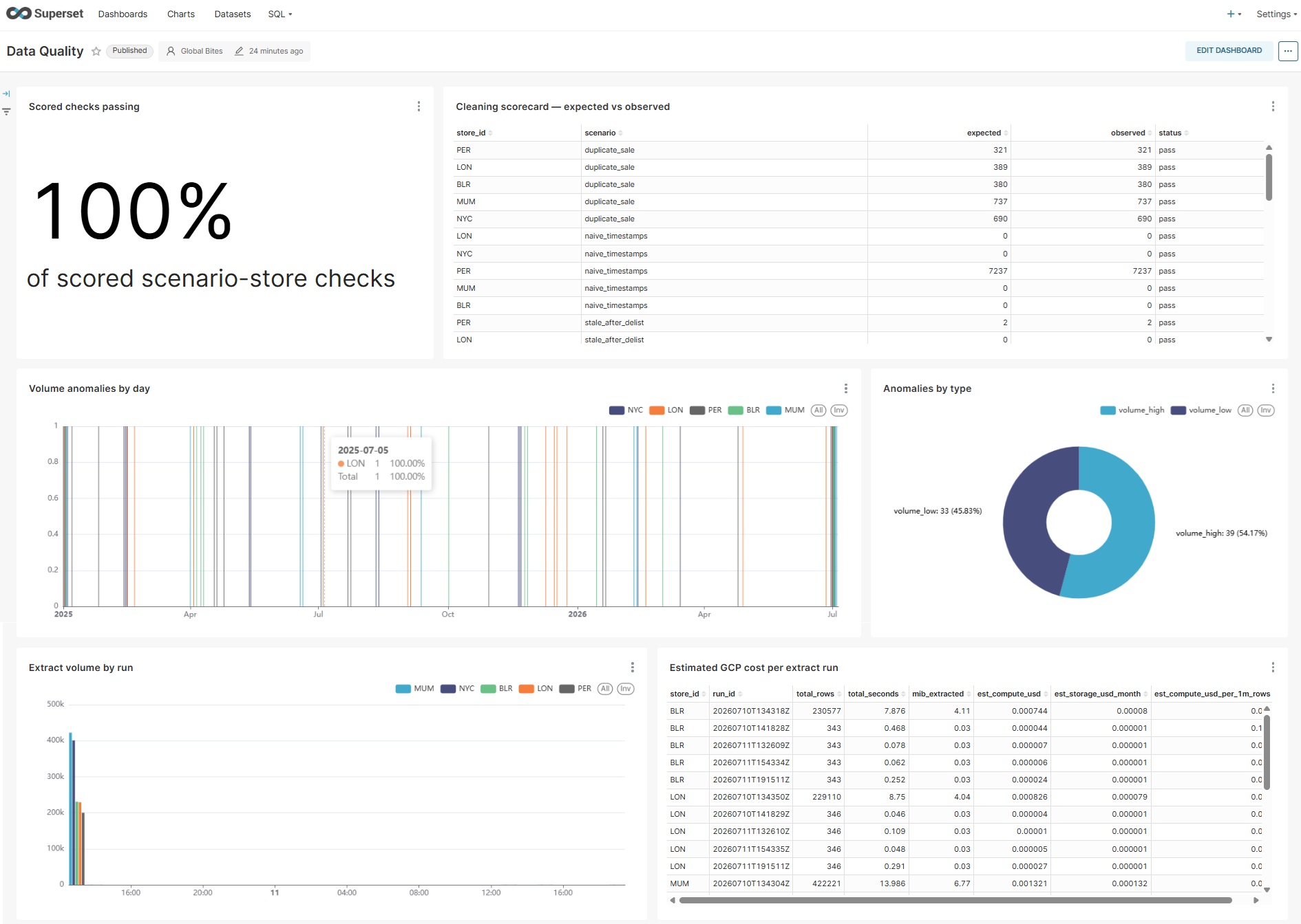
The ops layer is our favourite part: the pipeline watches itself. ops_extract_runs records throughput per extract, ops_volume_anomalies flags arrival-volume outliers against a 28-day median, and ops_cost_estimate prices every run as if it ran on cloud infrastructure, using a rate-card seed — so a price change is a data update, not a code change.
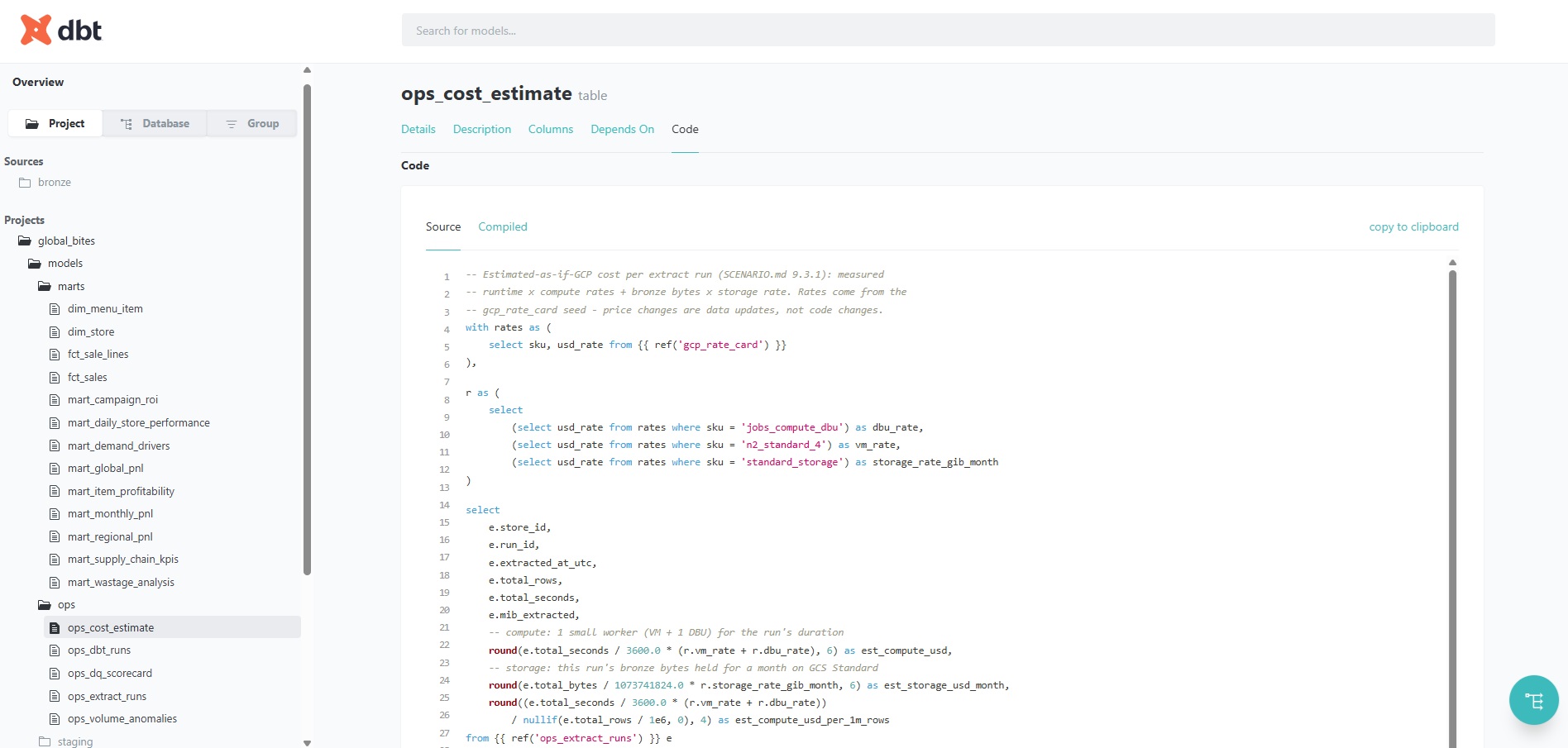
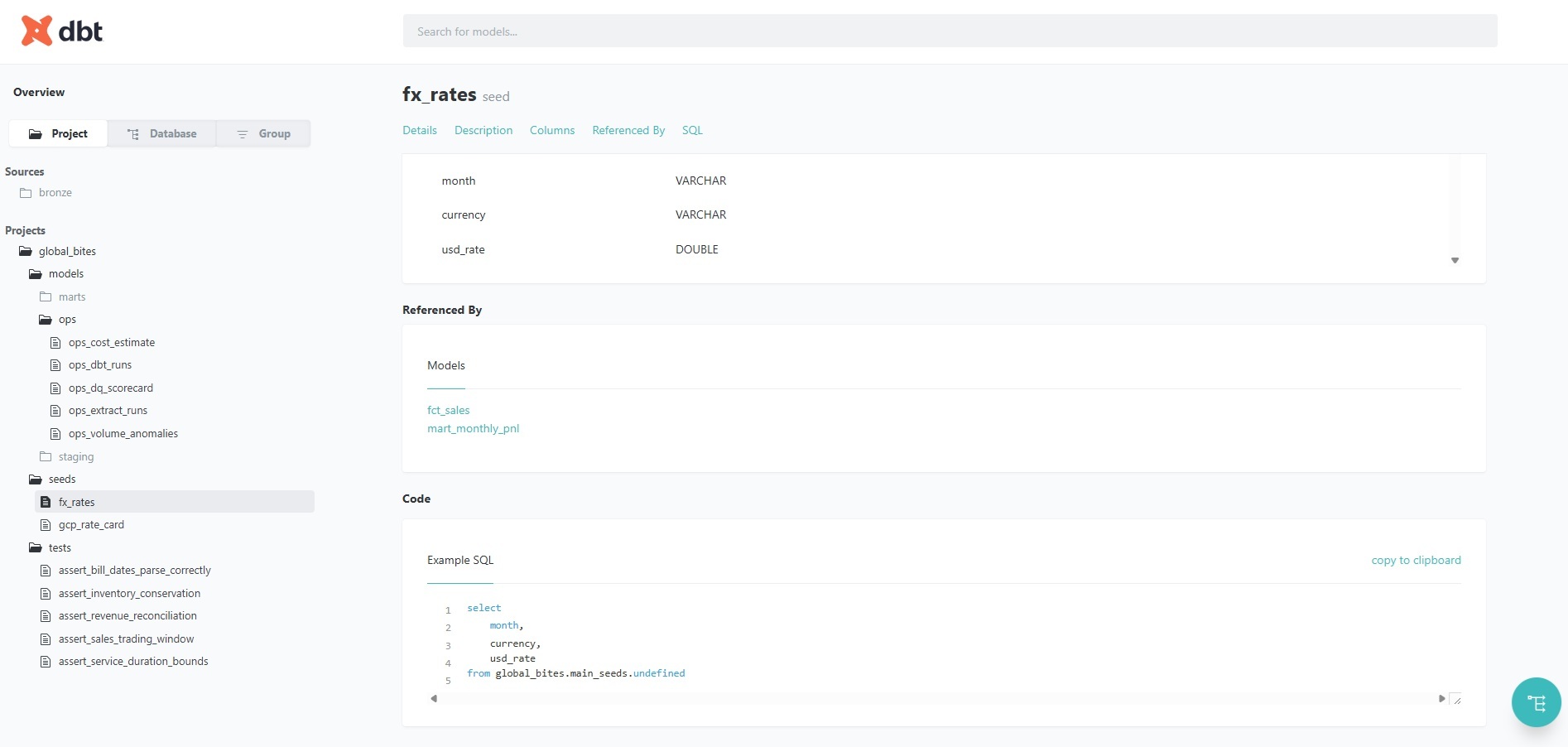
Seeds and tests are first-class citizens with the same lineage treatment. The fx_rates seed is referenced by the sales facts and the monthly P&L; the singular tests read like business rules because they are business rules — inventory conservation, a 10:00-to-20:00 trading window, service-duration bounds, and a revenue reconciliation of cleaned sales against each store's own day summary.
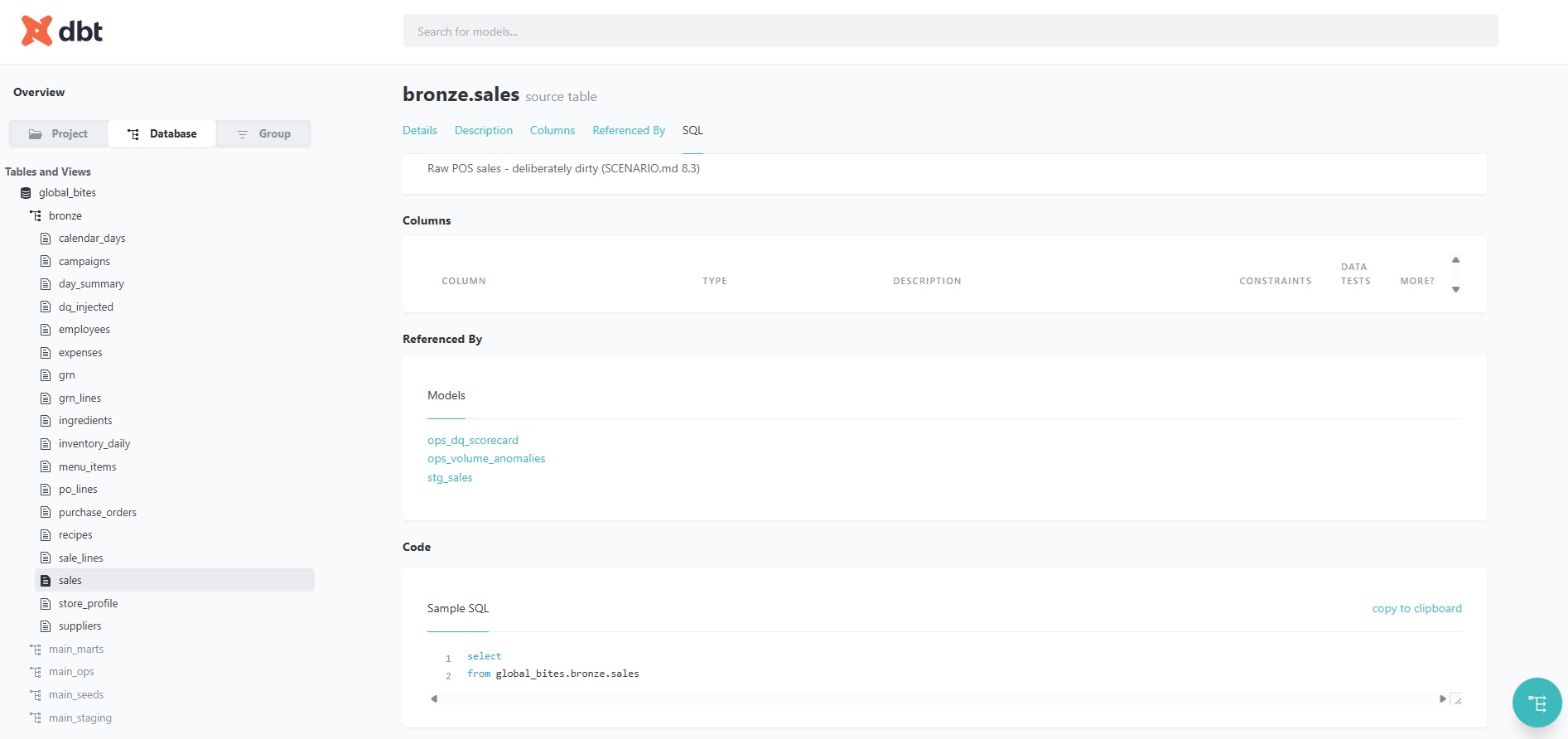
Lineage runs all the way down to the raw sources. The bronze sales table is documented as what it is — deliberately dirty POS data — and the docs show exactly which models consume it, so "where does this number come from?" has a clickable answer.
The cleaning, scenario by scenario
Thirteen distinct fault classes were injected into the source data — fourteen counting the regional date-format trap — and every one is handled in the dbt staging layer. Two principles govern all of it. First, the ground-truth manifest is only ever used to score the cleaning, never to perform it — anything else would be circular. Second, cleaning never destroys information: every correction leaves a was_* or is_* flag behind, so data quality itself becomes something the dashboards can report on.
- Duplicate sales — POS retries write the same sale twice (~0.5% of rows). Staging deduplicates on the natural key, keeping the latest batch's survivor, and a uniqueness test proves it stays fixed. - Partial re-sends and outage days — one day was first delivered 60% complete, then re-sent in full; the later batch supersedes the first. Days that arrive late in bulk are flagged by the volume-anomaly monitor (arrival counts vs a trailing 28-day median). - Late-arriving facts{teal} — roughly 2% of sales land one to three days after the event. Watermarked extraction picks them up whenever they arrive, and each row carries an is_late_arriving flag rather than being silently merged. - Late-arriving dimensions{blue} — seasonal menu items and replacement staff appear in sales before their master record syncs. SCD2 effective-date joins resolve those early sales once the master lands, so no fact is orphaned. - Slowly changing dimensions{purple} — menu price revisions, annual raises, and quarterly ingredient contracts become valid_from / valid_to version ranges, so historical margins are costed with the prices that were true at the time. - Schema drift{pink} — the delivery_channel column only exists from October 2025, and a gift_card tender appears in January 2026. Typed, nullable pass-throughs admit the new values without breaking a single older model. - Malformed values — totals arriving as strings with currency symbols and whitespace, null or inconsistently cased payment methods. Regex clean-up and typed casts yield a decimal total on every row, verified by a not-null test and an exact revenue reconciliation. - Regional date formats — the legacy billing feed writes dates as DD-MM in India, MM/DD in New York, and DD/MM in Perth and London: genuinely ambiguous for any day up to the 12th. Dates are parsed by the store's country, never guessed from the value, and a dedicated test fails on any mixup. - Timezone traps — two months of Perth sales carry naive local timestamps with no UTC at all. The pipeline reconstructs UTC from the store's fixed +08:00 offset — 7,281 rows repaired and verified against ground truth. - Refunds and voids — statuses are normalised and only completed sales count as revenue, while refund and void counts still flow through to the daily marts, because they are business signal, not noise. - Restatements — utility bills revised the following month and monthly stocktake adjustments: the latest revision wins, and a was_restated flag preserves the audit trail. - Referential breaks — sales recorded against a just-delisted item (a stale POS cache) resolve through the dimension's previous version and are flagged, not dropped. - Unit inconsistency — three months of Bangalore goods receipts reported produce in kilograms against gram-denominated masters. Quantities are normalised back to grams, with a was_kg_reported flag keeping the trail. - Orphan goods receipts — emergency purchases with no purchase order behind them are tolerated by design, flagged, and excluded from supplier on-time metrics, where they would be meaningless.
Beneath the scenarios sit two cross-cutting rules: every staging model deduplicates on its natural key — the guard that makes crash-retry re-extraction safe — and every event is re-anchored to a canonical UTC + local + offset triple, with business dates on the store's local trading day. Seven of the scenarios are scored exactly against the manifest and pass in all five stores; the rest are either corrected with the trail preserved or deliberately surfaced instead of erased.
Data quality is scored, not assumed
Because every injected fault was recorded in a ground-truth manifest, the pipeline's cleaning can be graded like an exam. The ops_dq_scorecard model compares what the staging layer found — duplicates removed, timestamps reconstructed, stale rows flagged — against what the manifest says was injected, per scenario, per store.
The scorecard currently reads 100% of scored scenario-store checks passing, across all five stores. That number is the honest version of "the data is clean": not a promise, a measurement. The same dashboard tracks volume anomalies by day, extract throughput, and the estimated cost of every run.
The payoff: seven dashboards, all of them code
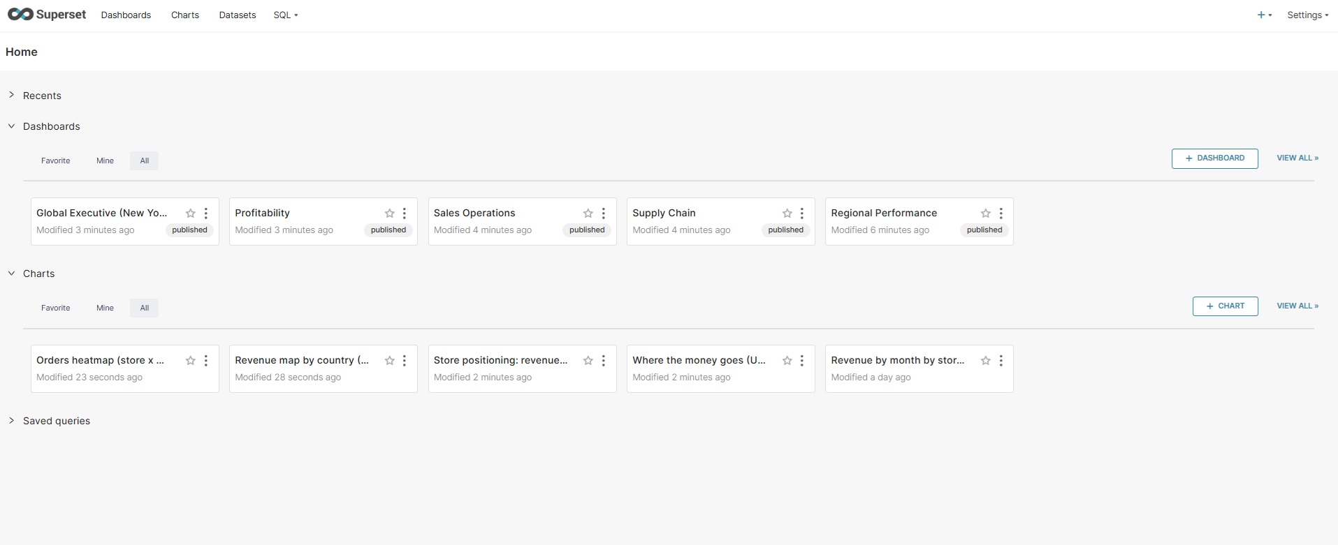
BI is Apache Superset, running as one more container beside the database. The seven dashboards are not click-ops: six are compiled from a spec that introspects the warehouse schema, the seventh is hand-authored YAML, and the whole bundle imports automatically on boot. A rebuilt Superset instance comes up with every dashboard already published.
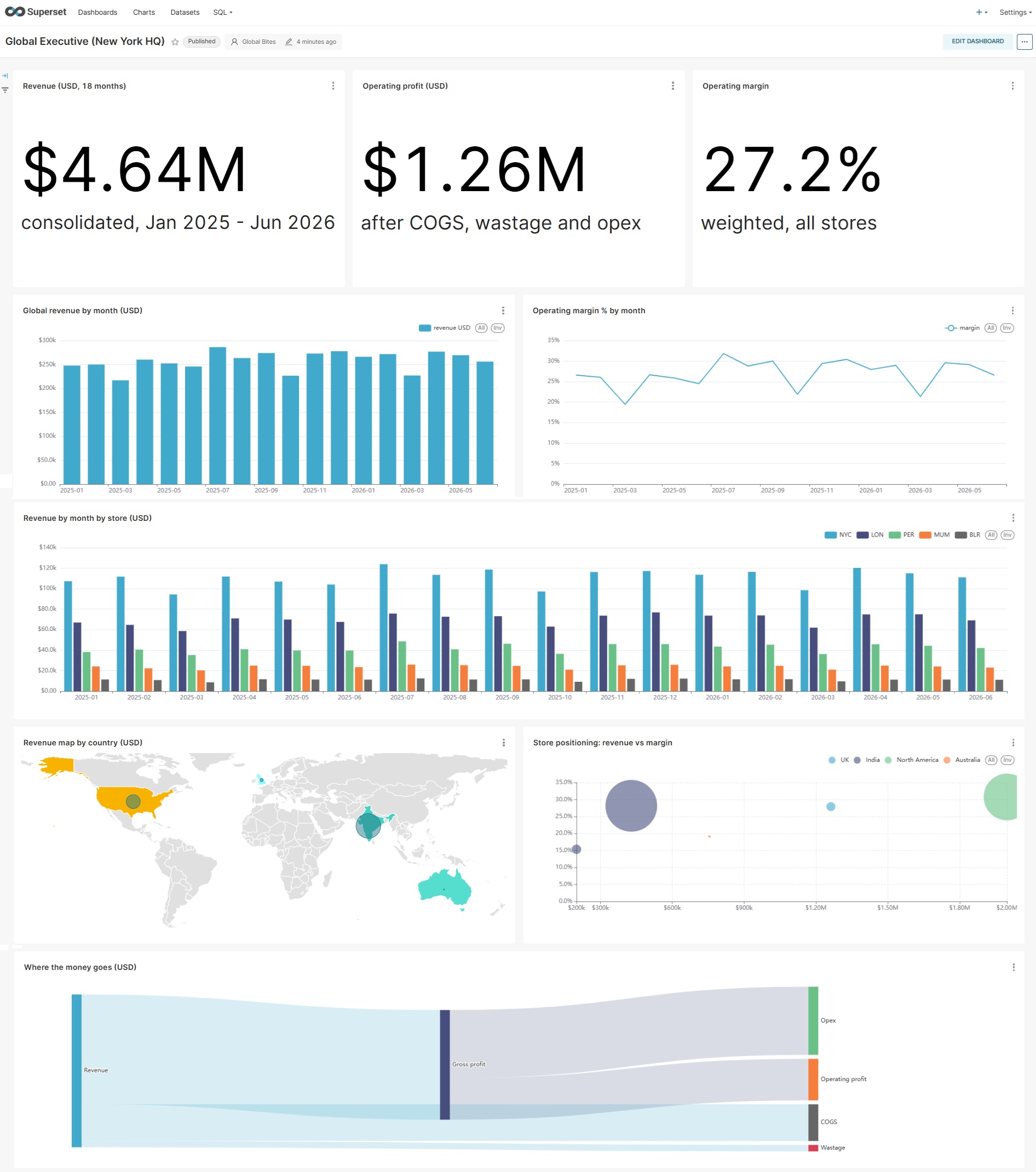
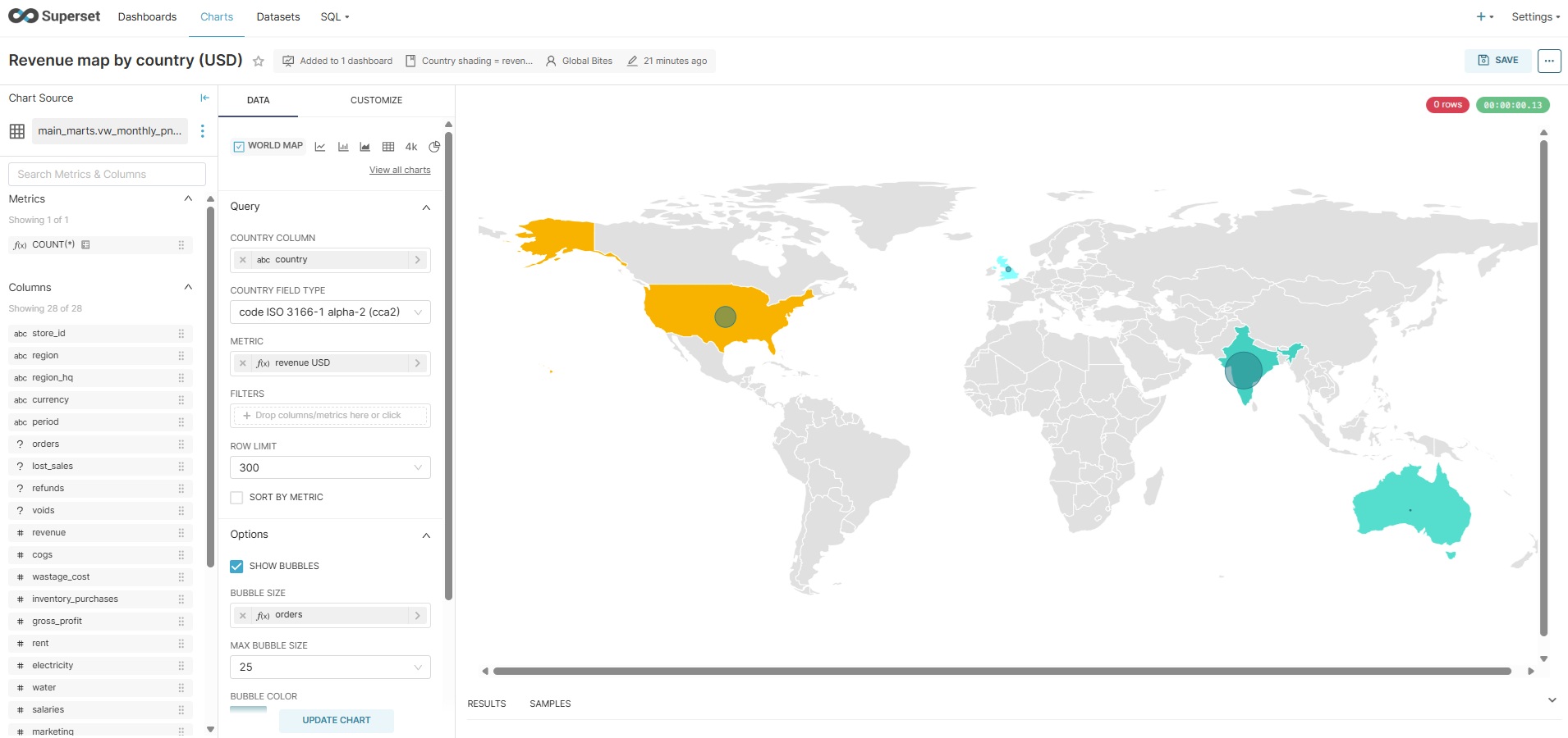
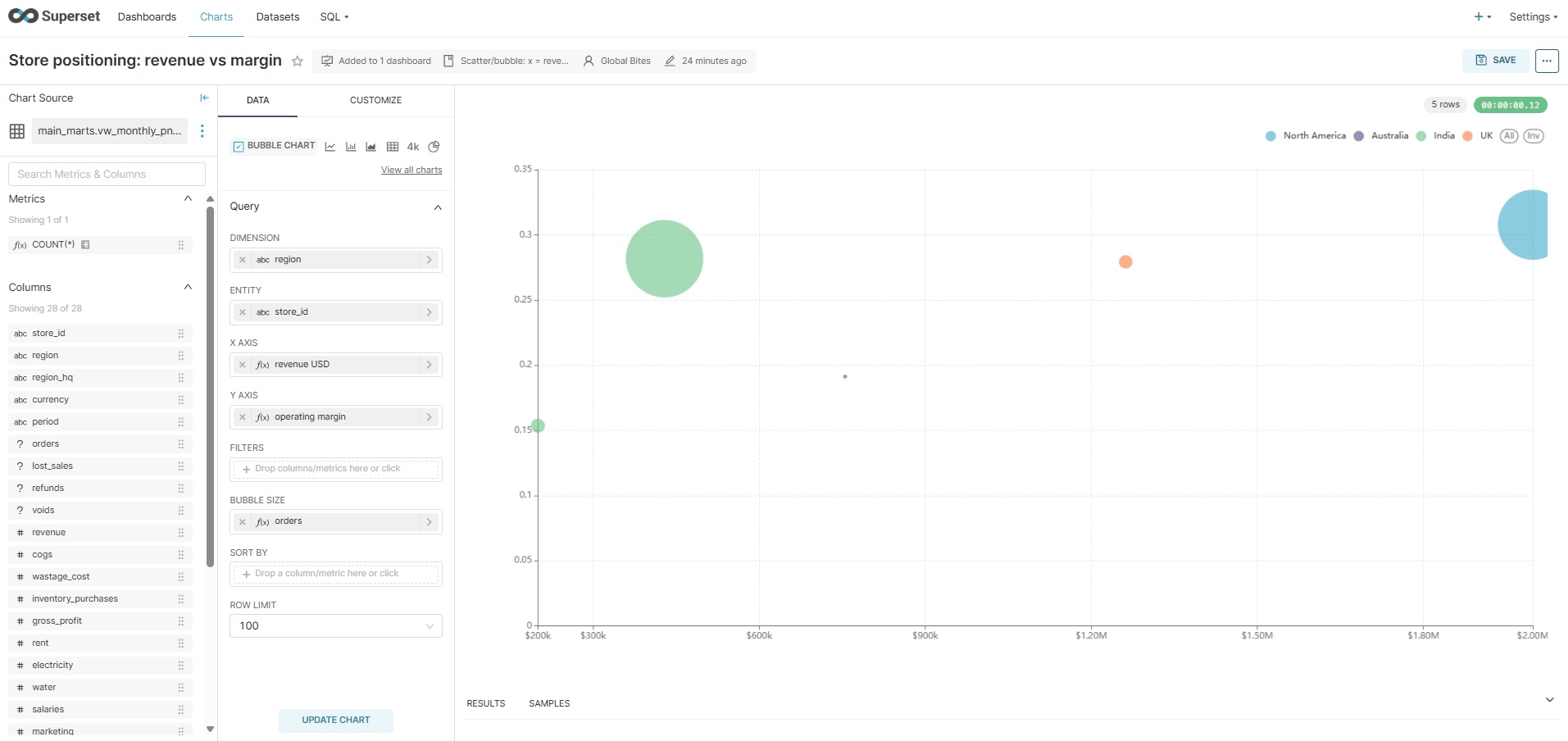
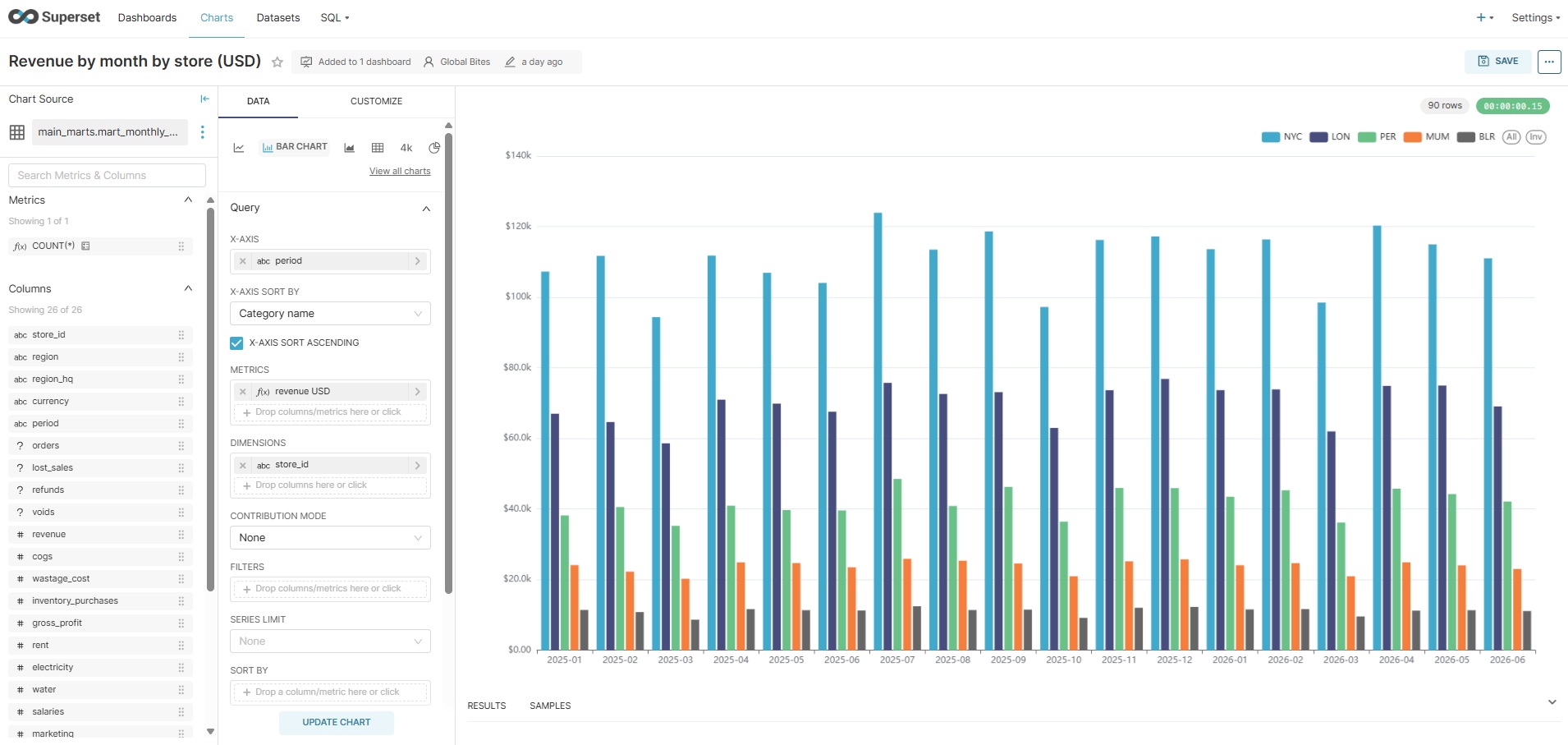
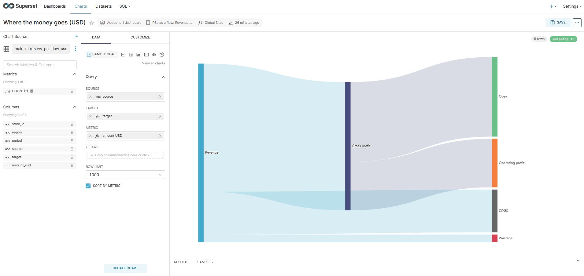
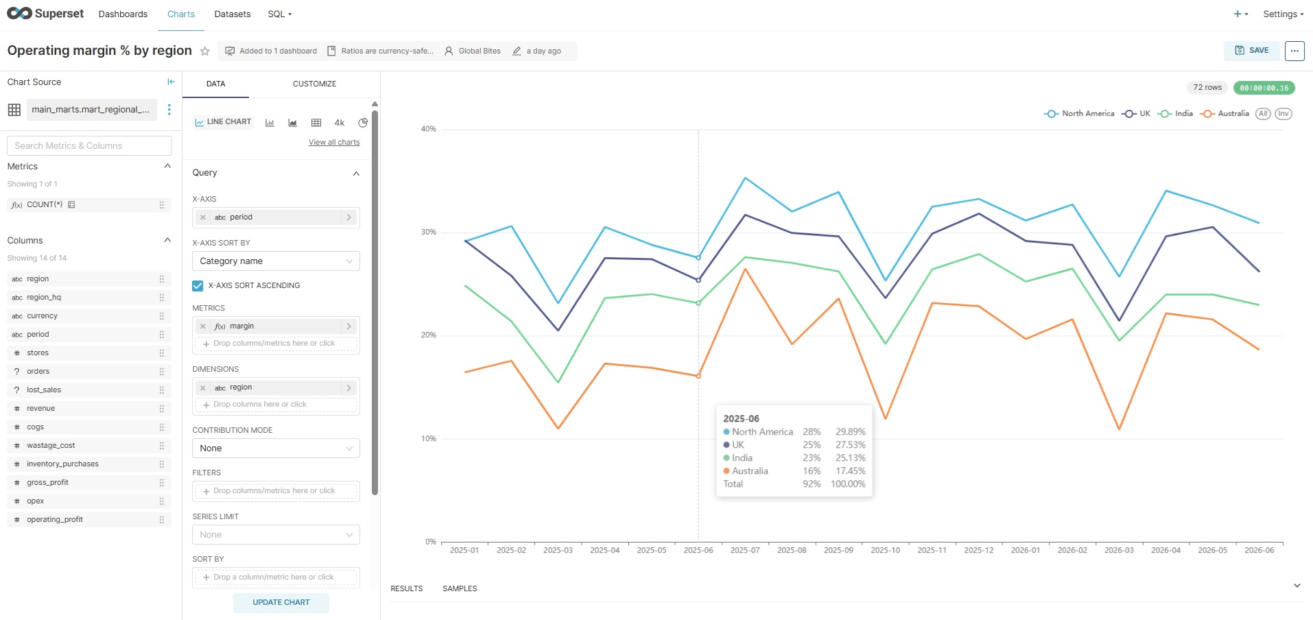
The Global Executive view is the consolidated HQ picture in USD: $4.64M revenue over the eighteen months, $1.26M operating profit, a 27.2% weighted operating margin — with monthly trends, a revenue map across the four countries, a store-positioning scatter of revenue against margin, and a Sankey showing where each revenue dollar ends up.
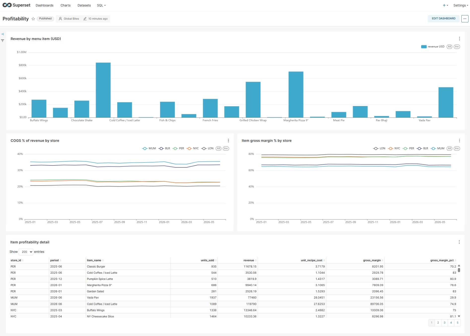
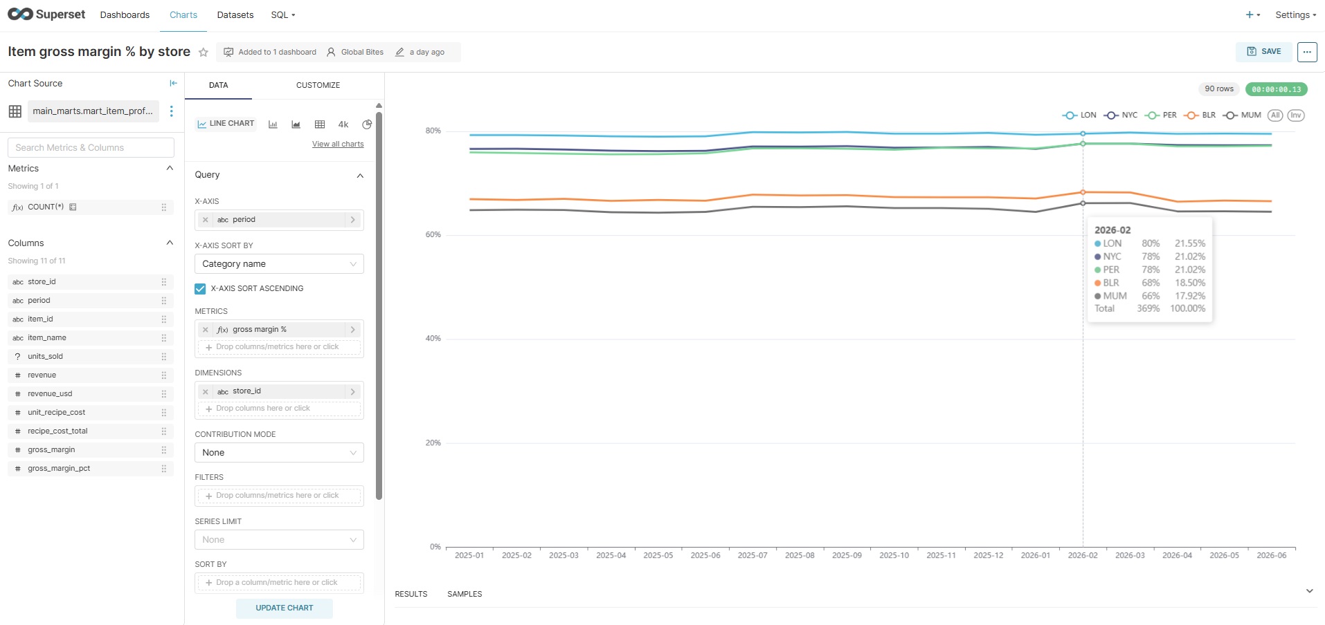
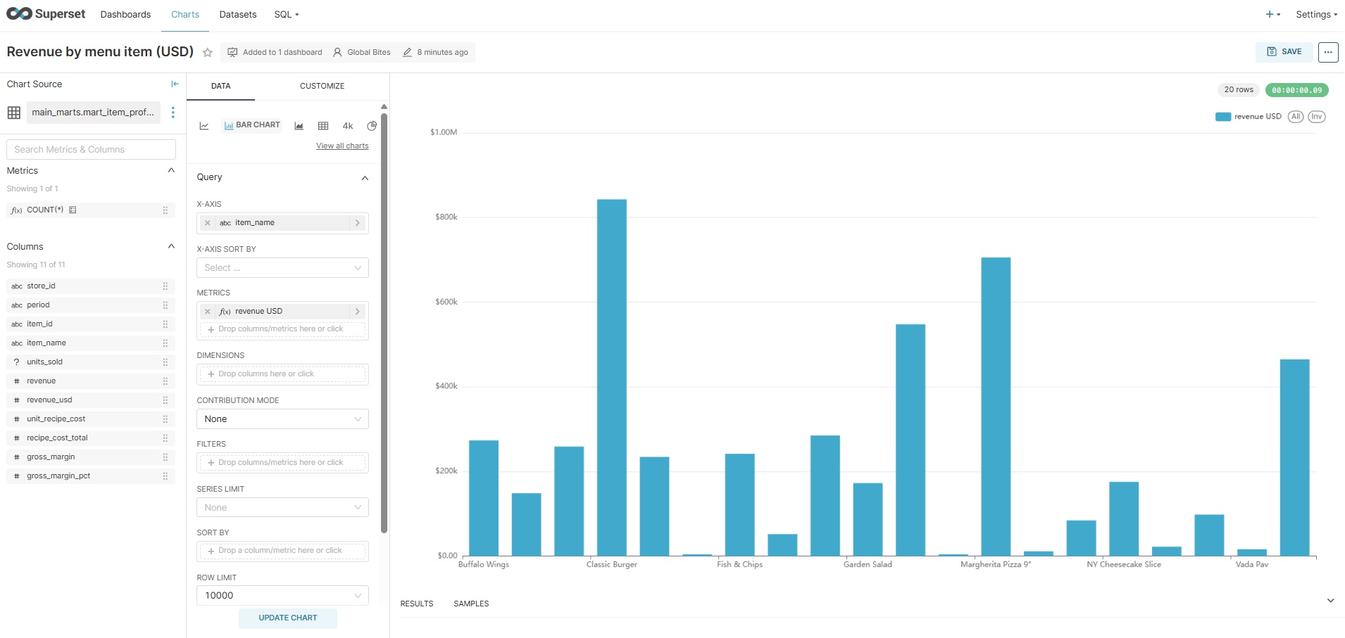
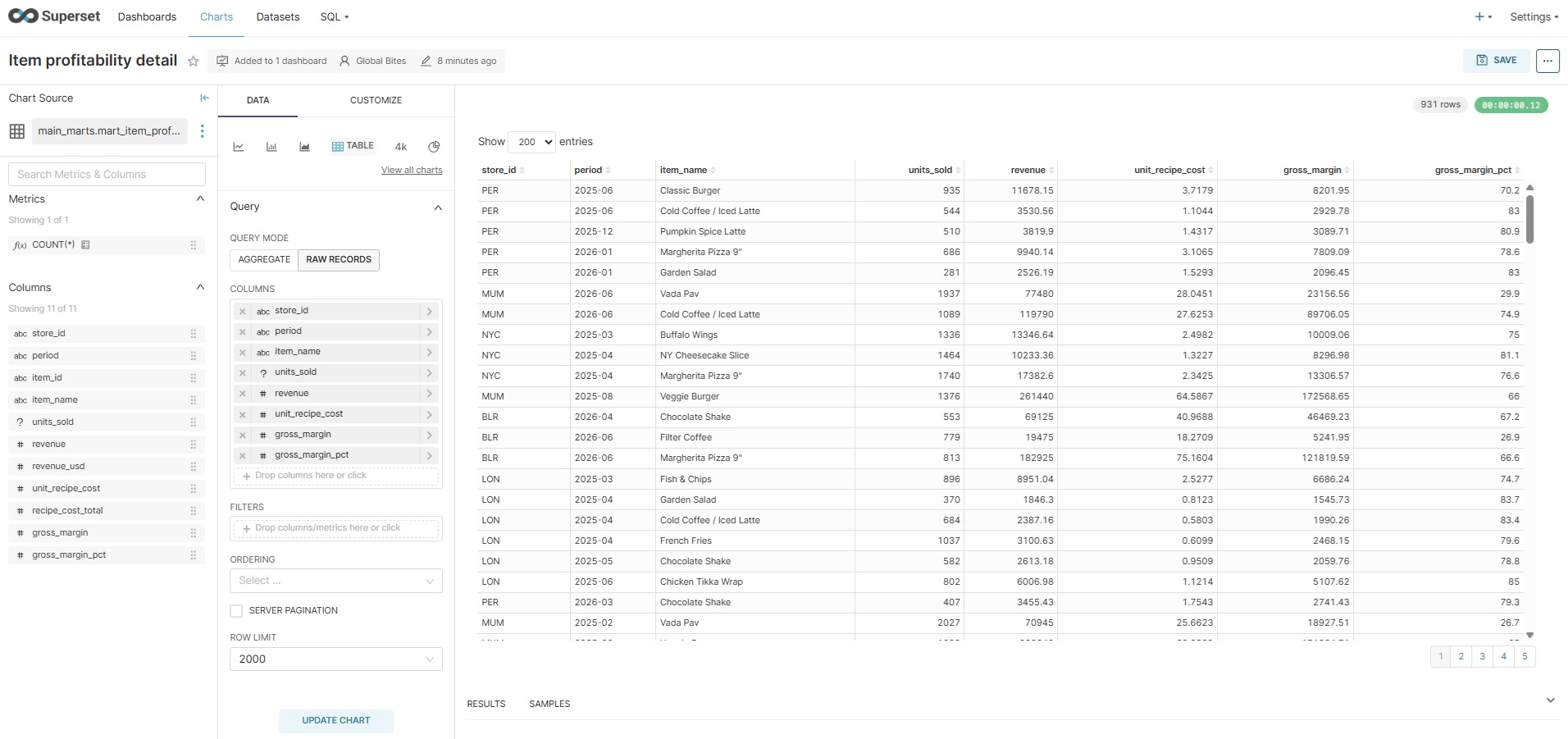
Profitability drills from menu-item revenue through COGS percentage by store to item-level gross margins, ending in a sortable detail table — the view a category manager would actually use to decide what stays on the menu.
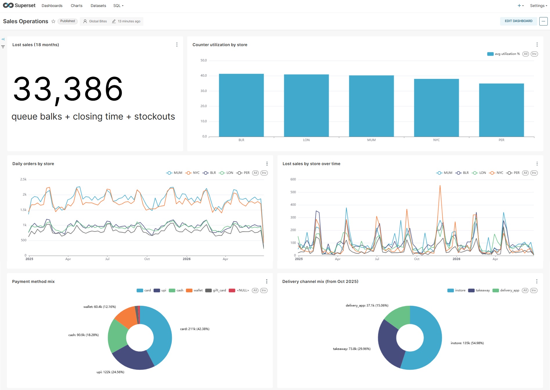
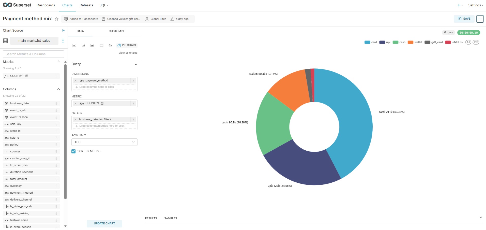
Sales Operations is the floor-level view: 33,386 lost sales decomposed into queue balks, closing-time misses, and stockouts, counter utilisation by store, daily order volumes, and the payment and delivery-channel mix — including the gift-card tender and delivery-app channel that only appear partway through the timeline, exactly as the source data introduced them.
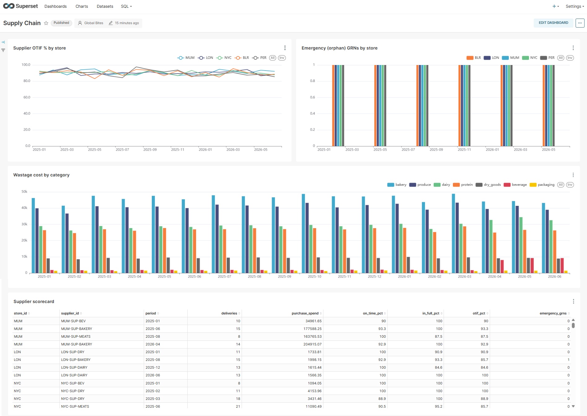
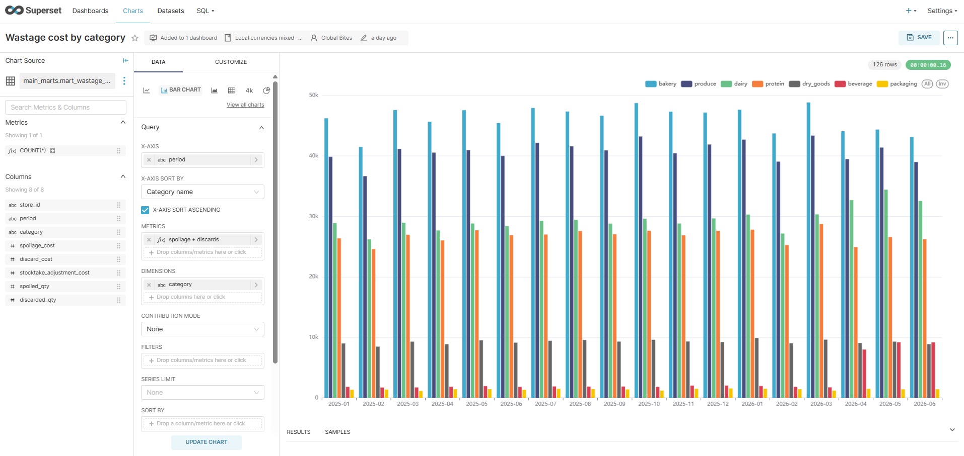
Supply Chain tracks supplier OTIF percentages, flags emergency goods receipts that arrived with no matching purchase order, and breaks wastage cost down by category, with a full supplier scorecard underneath.
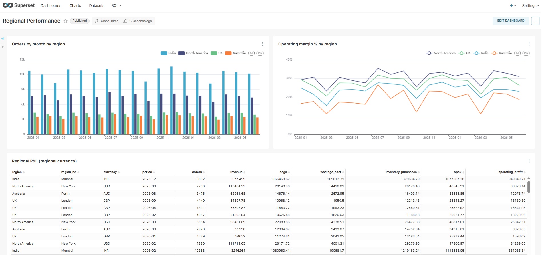
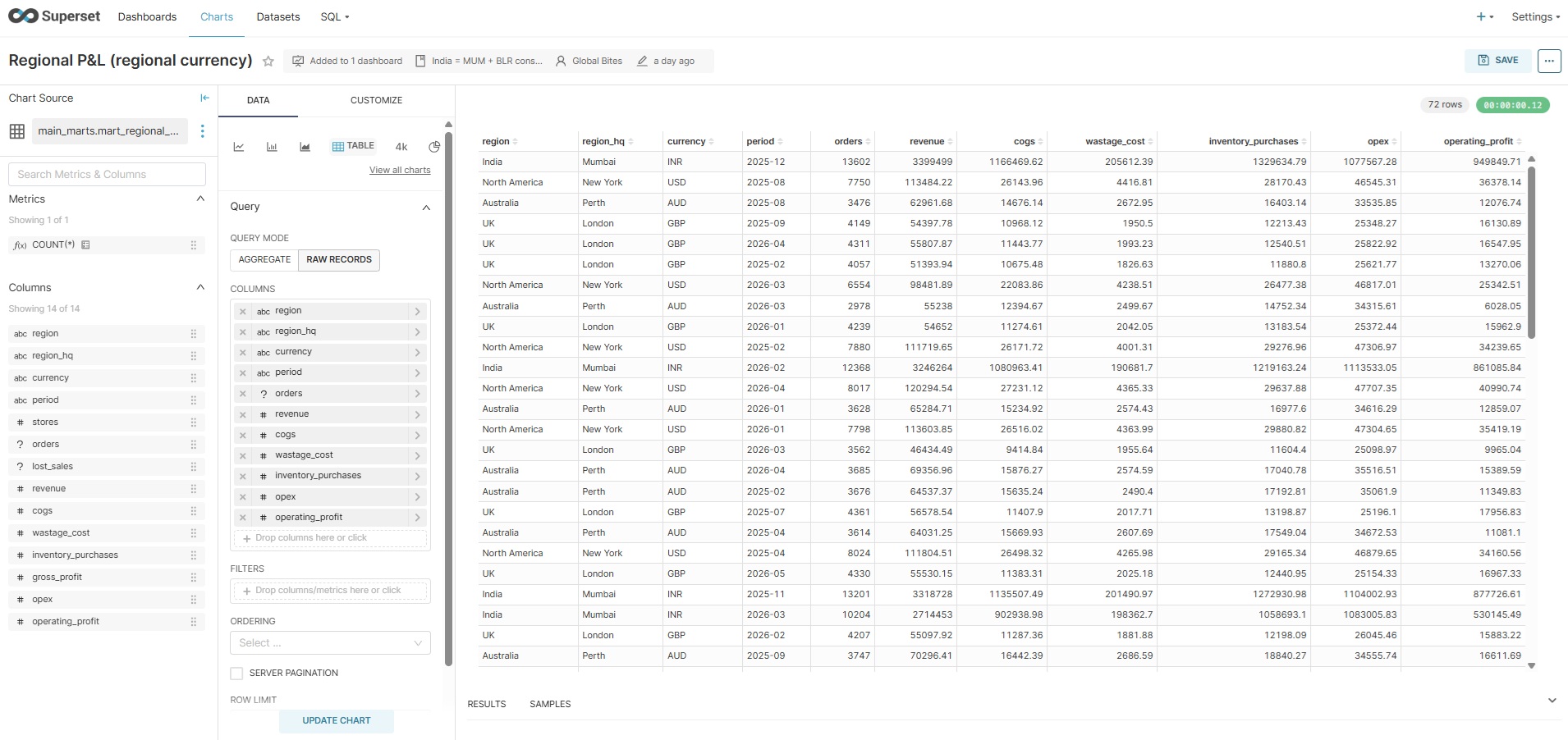
Regional Performance answers the question every multi-region business argues about: how each region is really doing, in its own currency. India reports Mumbai and Bangalore together in INR; the P&L table includes inventory purchases so regional managers see cash reality, not just accounting gross margin.
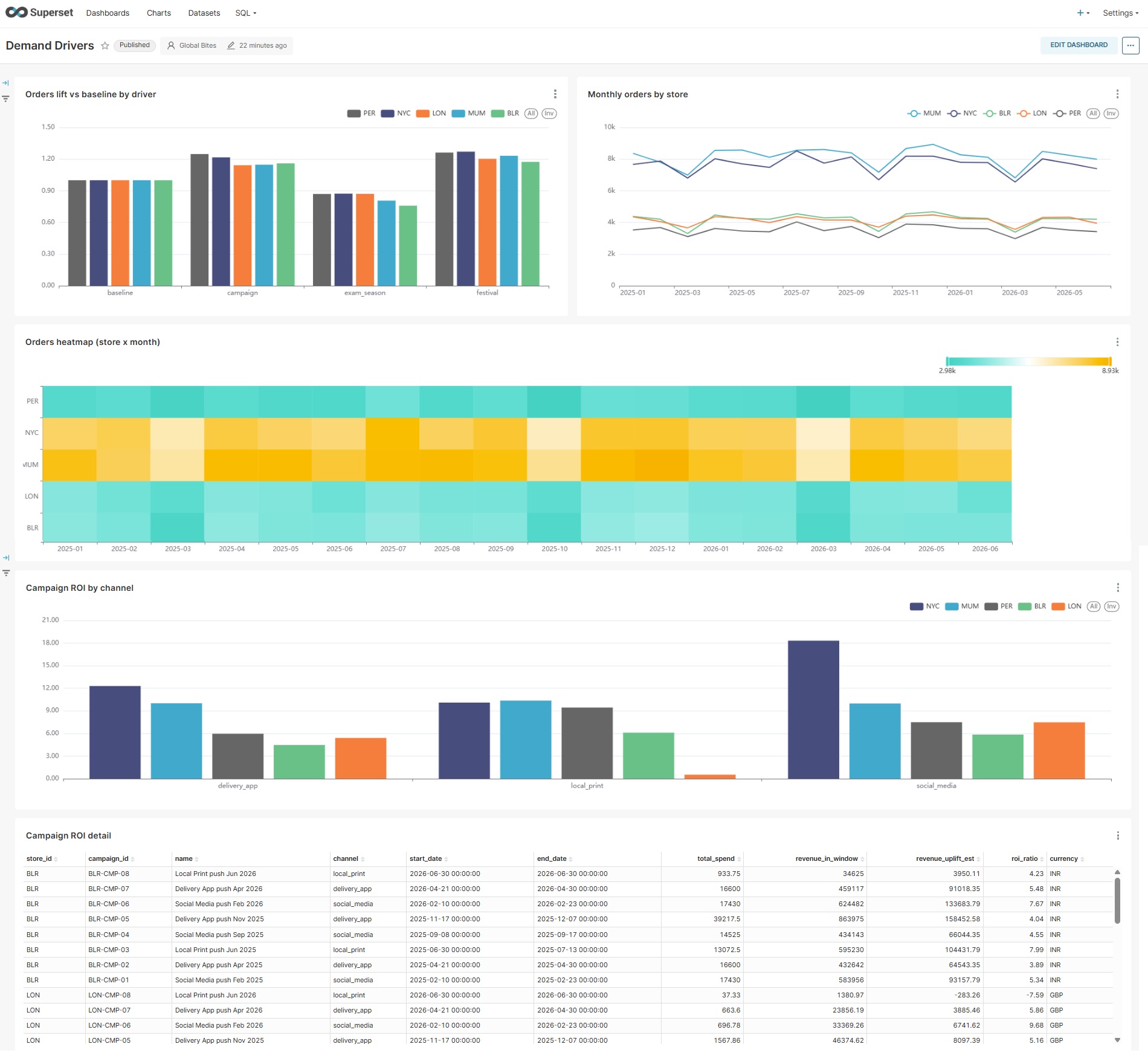
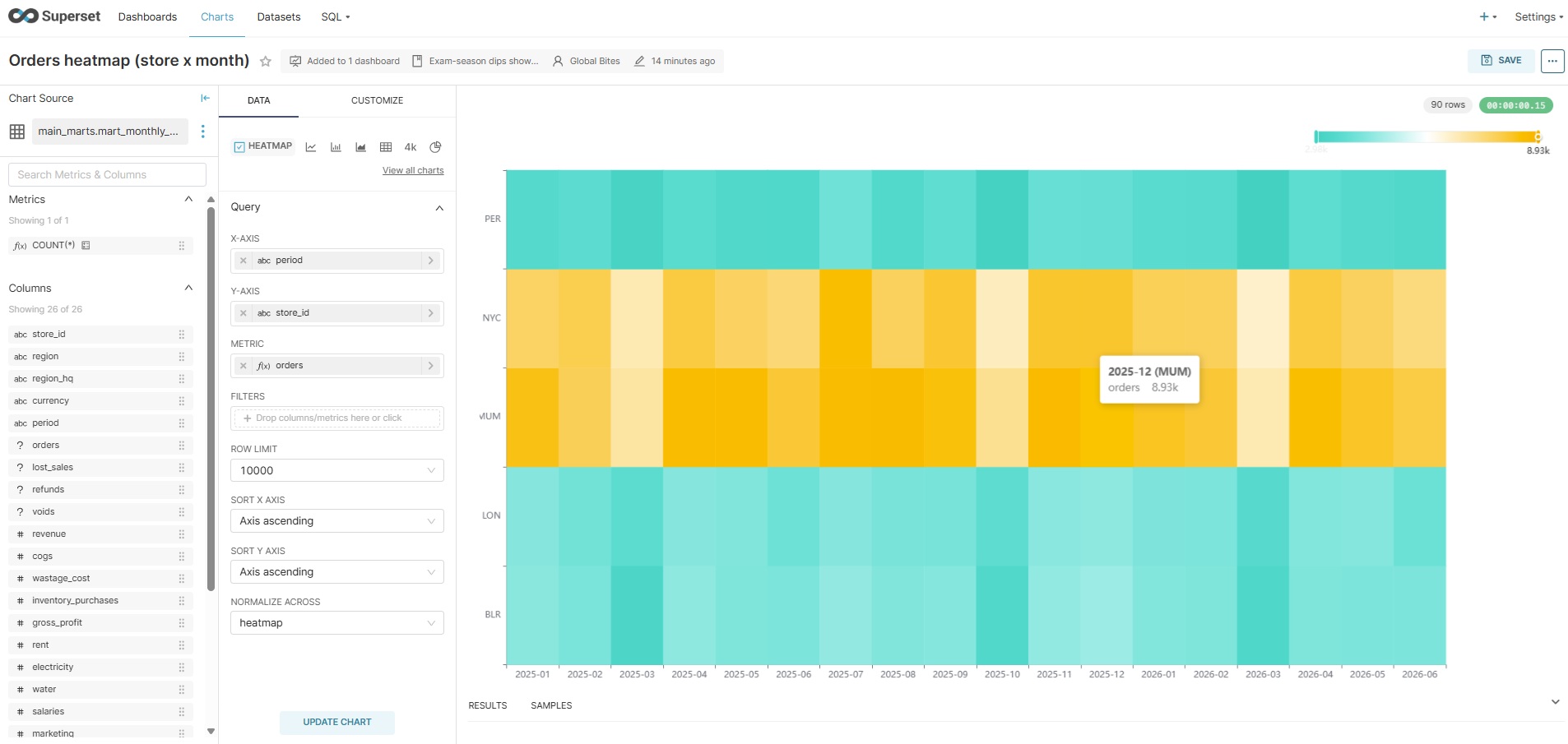
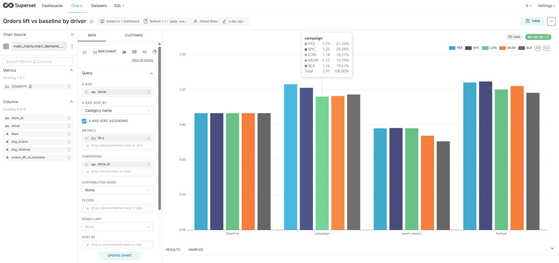
Demand Drivers separates signal from noise in the order volumes: festival and campaign lift versus baseline, exam-season dips, a store-by-month order heatmap, and campaign ROI by channel with the per-campaign detail to back it up.
A closer look at the charts
A few of the individual charts reward a full-size look — they carry most of the analytical story on their own.
What this build proves
Free, open-source tooling covers the entire path from raw operational databases to executive dashboards — Airflow, Parquet, dbt Core, DuckDB, and Superset left nothing missing. The constraint that mattered was never licence cost; it was engineering discipline.
Every layer is code. The DAG is seventy lines of reviewed Python, the warehouse is version-controlled SQL with tests, and even the dashboards are compiled from a spec and imported at boot. Rebuilding the whole platform from a fresh checkout is a runbook, not an archaeology project.
Every stage is idempotent: watermarked extracts re-land safely, staging deduplicates on natural keys, and dbt rebuilds from source on every run — so retries and backfills are safe by construction, which is exactly why that amber up_for_retry screenshot ends green.
And quality is measured, not asserted: dbt's tests gate the DAG, and the cleaning is scored against ground truth at 100%. That, ultimately, is what makes the dashboards worth trusting — every number on them can be traced back through tested, documented models to the raw rows it came from.